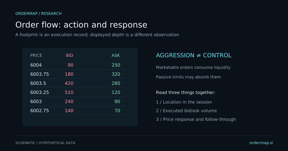
A liquidity heatmap places price on one axis and time on another, using color intensity to represent displayed resting quantity. It makes persistence, movement, and removal of visible liquidity easier to observe than a ladder that constantly updates. The color records a measurement under a chosen scale, not the confidence or identity of the trader behind an order.
A bright band can attract attention because it shows substantial displayed interest relative to the chart's scale. It does not promise that the size will remain when price arrives. Orders can be modified or canceled, and undisplayed interest may exist elsewhere. A heatmap is a view of a changing public book, not a complete inventory ledger.
Schematic only. A production heatmap would require timestamped book updates and an explicit depth range, neither of which is represented as live data here.
Visible size can be added, canceled, reduced by executions, or replaced through a sequence of updates. These changes can look similar in a compressed picture. A disappearing band is not enough to decide whether liquidity traded or was withdrawn. Pair book events with the transaction stream and account for the feed's sequencing rules.
Heatmap observation
What may have happened
What to verify
Bright band persists
Orders remain visible near a price
Whether size is static or replenishing
Band vanishes before contact
Cancellation or modification
Trades and ordered book updates
Large trades occur into a band
Displayed or replenished liquidity executes
Whether price progresses afterward
Size follows price
Orders are being moved or replaced
Event history, rather than one screenshot
The CME market-by-order overview explains the added granularity of anonymous order-level data. Market-by-price feeds aggregate size at each level. The available feed constrains what conclusions a heatmap can support.
Automatic normalization can make modest liquidity appear bright during a quiet period and substantial liquidity appear ordinary during a busy period. A fixed scale improves comparability but may hide smaller structures. Neither setting is inherently wrong; the reader needs to know which is in use.
Depth range matters too. A feed or chart showing a limited number of levels cannot establish that there is no liquidity beyond that range. Historical heatmap coverage may begin only when capture started. Blank space can mean unavailable data rather than an empty book.
Record whether the chart uses absolute quantities, relative intensity, smoothing, aggregation, or filtering. Avoid comparing screenshots from two products until those settings and data scopes are matched. Different colors are often a presentation difference rather than a disagreement about the market.
Suppose an invented market approaches a persistent offer band at 102. One scenario is rejection: aggressive buying arrives, price makes little progress, and then returns below the approach area. Another is acceptance: the offer trades or disappears, price holds above 102, and new transactions accumulate there.
The same bright band can precede either outcome. Define which sequence matters before contact. If your rule requires a retest, a one-way move without a retest is a missed observation under the rule, not permission to invent an earlier entry from the closing chart.
Avoid labeling routine cancellations as manipulation. Intent cannot be read from a colored line alone. The practical trading question is often simpler: how much visible liquidity remained, how much actually traded, and what did price do afterward? Those observations are useful without making legal or psychological claims.
Displayed quantity is not a guarantee that your order would execute. Queue position, matching rules, latency, cancellations, and competing orders affect fills. A hypothetical limit order placed at a historical bright band should not automatically receive a perfect simulated fill merely because price touched the level.
CME's Liquidity Tool separates bid-ask spread, depth, and cost to trade. That separation is useful: a tight spread can coexist with limited size, and deep visible size can disappear during stress. Evaluate the execution assumption separately from the analytics signal.
Choose twenty approaches to a preidentified liquidity region. Save the book context, the transaction sequence, and what happened after contact. Classify added, canceled, traded, and unclear activity. Keep uncertain cases rather than forcing them into a persuasive category.
Compare heatmap observations with a price-and-volume baseline. Did the historical depth add useful information before the outcome? Did it encourage premature fading? Did normalization or missing capture change your impression? These questions turn an attractive visual into a disciplined research tool.
Consider an invented offer band of 500 contracts at 102. It disappears just before price reaches that level. If only 20 contracts executed there during the relevant sequence, describing all 500 as consumed would be unsupported. Cancellations, modifications, and changes in aggregation may explain much of the disappearance.
Now consider 800 contracts executing while visible size repeatedly returns near 500. This is a different observation: substantial trading and replenishment occurred. Even then, the total does not prove one owner or a fixed original hidden size.
For a practical exercise, replay a short interval slowly and write a chronology of displayed size and trades. Mark uncertain ordering instead of guessing. Then compare your event notes with the compressed heatmap. The exercise reveals which conclusions the visual supports directly and which require details that may be lost through sampling, normalization, or incomplete capture.